JobsEQ now includes preliminary estimates for occupation wages in order to provide timely compensation data. These data build upon the BLS OEWS data set.
Workforce
Data
Economy
JobsEQ
Trends
Analysis

By Chmura Economics & Analytics
Published Jan 27, 2023
JobsEQ now includes preliminary estimates for occupation wages in order to provide a more timely compensation data set. These data build upon the Bureau of Labor Statistic’s (BLS) OEWS[1] data set which produces wages data for detailed occupations[2] at the state and metropolitan area level.
The BLS collects data from local employers to create the valuable OEWS wages estimates. However, the process of collecting and compiling these survey-based data creates a ten-month time-lag between the reference period of the data and their publication. This is especially an issue for occupation wage data which can become stale with time, particularly in an economic environment of elevated wage inflation. These data are also only updated once a year, further impacting the real-time time lag.
To narrow the time gap, JobsEQ combines other compensation data from the BLS along with wage information collected from our real-time job ads data set (RTI) to project the OEWS data forward. This process makes the JobsEQ occupation wages data set about one year more current than it would be otherwise.
To measure the accuracy of these wage projections (see below for more details), preliminary estimates for one year into the future were compared against the baseline of using the prior year’s data as an estimate for the subsequent year.[3] For state-occupation combinations with a large employment base,[4] the median error was reduced by 49% by using our projected wages. Specifically, the median error for the baseline method was 3.11% compared to 1.58% for our projections.
Our estimation method was also compared to bringing forward wages via the Consumer Price Index (CPI) or using average wage changes from the Quarterly Census of Employment and Wages (QCEW); in both cases our method provided better results.
Technical Notes: Accuracy and OEWS as a Time-Series
A problematic and important element in testing wage forecasts against OEWS data is that these data were not designed for time comparisons, as the BLS is clear to disclose: “The Bureau of Labor Statistics at present does not use or encourage the use of OEWS data for time-series analysis.” And again: “Although the OEWS survey methodology is designed to create detailed cross-sectional employment and wage estimates by geographic area or industry, it is less useful for comparing two or more points in time.”[5]
Besides methodological and classification definition changes that can impact comparisons over time, the OEWS data set is based on survey data that can have sampling errors that are large relative to the amount of change being observed over time, thus undercutting the time analysis.
Therefore, while the OEWS data are valuable point-in-time estimates, use of these data in a time-series must be done cautiously. The below chart illustrates the issue:
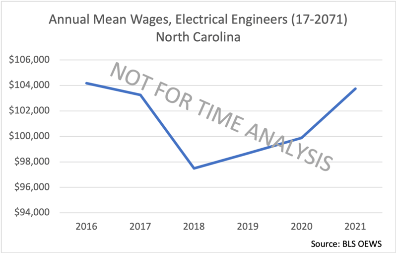
First off, apologies to the BLS because even creating and displaying this line chart for these data is a bit unfair as it presents these data as a time-series. This is the very view that the BLS cautions against as the data were not created for this type of presentation.
Nevertheless, for purposes of illustration, if we were to view these data as a time series we’d see some surprising changes year-to-year. Electrical engineers in North Carolina averaged about 5,000 employment during this period, and for such a large group we’d expect to see a fairly moderate and steadily upward rate of growth in average wages over time. Instead, we see a couple year-to-year declines—including a large drop in 2018—as well as a larger-than-expected increase in 2021. This volatility in estimates over time is what the BLS is cautioning about when using these data.
Furthermore, note that the above example is not the most extreme example of volatility in estimates over time in the OEWS data. This occupation-region combination is based on a fairly large employment base, meaning its survey sample size is likely larger and relative errors should be smaller. Alternatively, if we looked at—for example—the wages data for soil and plant scientists (SOC 19-1013) in Oklahoma, a unit where employment averages less than 200, we’d see more extreme examples of volatility in wage estimates.
This characteristic of the OEWS data creates a difficulty when using it to measure accuracy of a wage forecast, simply because the data set is problematic when used for time comparisons. This is why in the accuracy statistic used in the first portion of the article we used the subset of units that were based on 10,000 or more in employment as those units tend to have more stability for time comparisons.[6]
-----------
[1] OEWS = Occupational Employment and Wage Statistics.
[2] “Detailed occupations” here refers to six-digit SOC codes (Standard Occupational Classification System).
[3] In other words, wages were forecast from a year of OEWS data to predict the subsequent year, with the error measured relative to the actual wages reported for the subsequent year. The baseline is using the prior year’s OEWS wage unchanged as an estimate for the next year.
[4] “Large employment base” means state-occupation unit where the employment of that unit was 10,000 or more. Over 11,000 such pairs were used for the statistic cited in the text, specifically, units from state-level and six-digit occupations between 2017 and 2021.
[5] See https://www.bls.gov/oes/oes_ques.htm for further details.
[6] All units with disclosed wage data were used in the accuracy analysis and improvement in that data set overall was found when tested. Differences in improvement measured, however, weren’t as large, due in-part to the increased volatility in the underlying data which had smaller average sample sizes.


